Let’s take a simple, visual approach to understanding vector math, starting with what you see on screen – the dots – and ending with the corrective actions you take.
The circular plot: where balancing begins
When balancing a rotating machine, we use a circular (or polar) plot to visualise vibration. This plot shows two key things:
-
Amplitude – how much the machine is vibrating, represented by the distance from the centre
-
Phase – when in the rotation the vibration occurs, shown as an angle around the circle

Your first reading: the reference run
Before making any changes, we collect a reference run – a reading of how the machine is currently behaving.
This data appears as a single orange dot on the circular plot. For instance:
-
If the dot is five segments away from the centre, and each segment represents 1 mil, then the amplitude is 5 mils
-
If the dot sits at 90°, then that’s your phase angle
It’s the starting point – your first ‘dot’.

Adding a trial weight: watching the plot move
Next, we apply a trial weight to the machine. This is not the final correction – it’s a test to see how the system reacts.
We follow the 30/30 rule:
-
The vibration should change by at least 30% in amplitude, or
-
Shift phase by at least 30 degrees
If we see either change, the trial is successful, and we can proceed to calculate the correction.
After the trial weight, a new blue dot appears on the plot, showing the machine’s updated vibration. Now we’ve got two dots – and that’s when the decisions begin.

The blue dot in the image above will represent the reading after applying the trial weight. At this point, we have enough information to make our correction
Understanding the math: connecting the dots
Let’s break it down visually:

If we had done this manually, the fuchsia-colored arrow would have been drawn on the plot. Then, we would get out a protractor to measure the angle and a ruler to measure the length. Using the formula (Length/Amplitude), we will get a number that can be expressed as Grams/Inches.
With that information, we will impose the angle and length of the fuchsia arrow on the orange dot, which was the original run or “reference run”. You can see that We did that here by adding the green arrow.

To keep the chart simple, I removed the trial run information.
The next step is to draw a line from the end of the green arrow to the center of the plot. At this point, we can measure the angle and length of the orange line.

We take the angle and length of the orange line and flip it 180 degrees to draw our red line and establish the point at which we need to place our correction weight and how much weight we need to apply.
By measuring the length of the line and using our values from earlier, as far as grams/inch or whatever the units may be, we can determine the amount of weight needed to make the correction.
This is the math that is taking place inside your data collector. By understanding this concept, you will have a better understanding of the balance process and be more capable of identifying errors before they occur.
From maths to machine: why it still matters
Even though your vibration analyser or wireless balancer performs these calculations automatically, understanding what’s happening behind the scenes helps you work smarter. You’ll be able to:
-
Spot incorrect data or faulty readings
-
Avoid over- or under-correction
-
Interpret results with greater confidence
Balancing made simple – with clarity and control
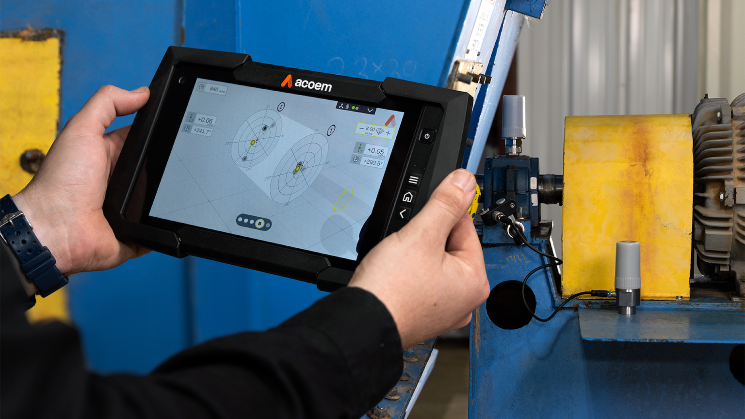
The Acoem Wireless Balancer takes care of the complex vector maths for you, delivering accurate results in real time. But it doesn’t hide the process – it gives you full visibility of every vector, every angle, and every decision point.
You get the best of both worlds:
-
Precision automation
-
Complete understanding